10.6. Solving Implicit Equations
An explicit function is written as the dependent variable defined in terms of the independent variables. Some examples are:
An implicit function is a function where the dependent variable is not defined in terms of the independent variables or constants. Some examples of implicit functions are:
Solving Implicit Equations
Some systems of implicit equations can be solved algebraically while some are easier to solve by graphing. Algebraically, the solution to a system of equations is the points that satisfy all equations. On a graph, the solution is the intersections of the curves.
To solve a system of implicit equations, type the equations as they appear in the problem with one equation per line. If no answer is shown, the system is easier to solve by graphing. In this case, switch to Graph mode.
Examples
Solve each system of implicit equations below.
Problem 1
Algebraic solution
Enter the first equation: 3x + 4y = 6. Type the variable y by tapping the x variable key twice. Hit enter.
Enter the second equation: x^2 + y^2 = 4.
Note: The answers shown are the values of the dependent variable y.
Enter the first equation: 3x + 4y = 6. Type the variable y by tapping the x variable key twice. Hit enter.
Enter the second equation: x^2 + y^2 = 4.
Note: The answers shown are the values of the dependent variable y.
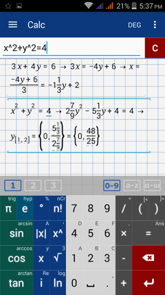
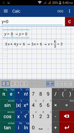
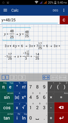
To find the corresponding values of the independent variable x, evaluate either the first or second equation at y = 0 and
y = 48/25 = 1.92. Type y = 0 and then the equation you want to use. E.g. y = 0, then 3x + 4y = 6. To find the value of x when y = 48/25, edit y = 0 and change 0 to 48/25.
y = 48/25 = 1.92. Type y = 0 and then the equation you want to use. E.g. y = 0, then 3x + 4y = 6. To find the value of x when y = 48/25, edit y = 0 and change 0 to 48/25.
Solution by Graphing
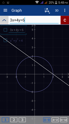
Switch to Graph mode by selecting Graph from the navigation menu.
Enter the first equation: 3x + 4y = 6. Type the variable y by tapping the x variable key twice. Hit enter.
Enter the second equation: x^2 + y^2 = 4.
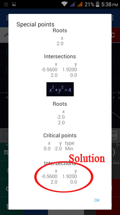
Tap the special points key. Check the "show intersections" option.
Tap "show all."
Switch to Graph mode by selecting Graph from the navigation menu.
Enter the first equation: 3x + 4y = 6. Type the variable y by tapping the x variable key twice. Hit enter.
Enter the second equation: x^2 + y^2 = 4.
Tap the special points key. Check the "show intersections" option.
Tap "show all."
Problem 2
Algebraic solution
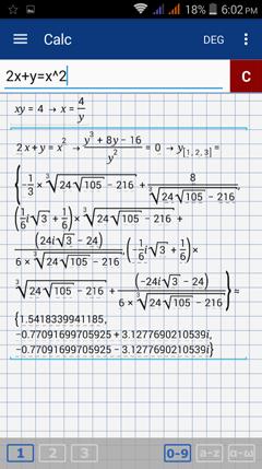
Enter the first equation: xy = 4. Type the variable y by tapping the x variable key twice. Hit enter.
Enter the second equation: 2x + y = x^2.
Note: The values of y shown are imaginary numbers so it's easier to solve the system of equations by graphing. See the graphical solution.
Enter the first equation: xy = 4. Type the variable y by tapping the x variable key twice. Hit enter.
Enter the second equation: 2x + y = x^2.
Note: The values of y shown are imaginary numbers so it's easier to solve the system of equations by graphing. See the graphical solution.
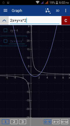
Solution by Graphing
Switch to Graph mode by selecting Graph from the navigation menu.
Enter the first equation: xy = 4. Type the variable y by tapping the x variable key twice. Hit enter.
Enter the second equation: 2x + y = x^2.
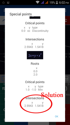
Tap the special points key. Check the "show intersections" option.
Tap "show all."
Switch to Graph mode by selecting Graph from the navigation menu.
Enter the first equation: xy = 4. Type the variable y by tapping the x variable key twice. Hit enter.
Enter the second equation: 2x + y = x^2.
Tap the special points key. Check the "show intersections" option.
Tap "show all."
Problem 3
Algebraic solution
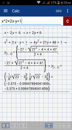
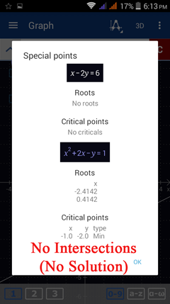
Enter the first equation: x - 2y = 6. Type the variable y by tapping the x variable key twice. Hit enter.
Enter the second equation: x^2 + 2x - y = 1.
Note: The values of y shown are imaginary numbers so it's easier to solve the system of equations by graphing.
Enter the first equation: x - 2y = 6. Type the variable y by tapping the x variable key twice. Hit enter.
Enter the second equation: x^2 + 2x - y = 1.
Note: The values of y shown are imaginary numbers so it's easier to solve the system of equations by graphing.
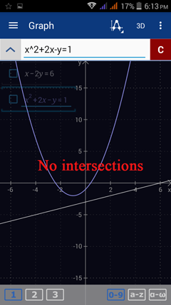
Solution by Graphing
Switch to Graph mode by selecting Graph from the navigation menu.
Enter the first equation: x - 2y = 6. Type the variable y by tapping the x variable key twice. Hit enter.
Enter the second equation: x^2 + 2x - y = 1.
Tap the special points key. Check the "show intersections" option.
Tap "show all."
Note: The two graphs do not intersect. There is no real number solution to the system of equations.
Problem 4
Algebraic solution
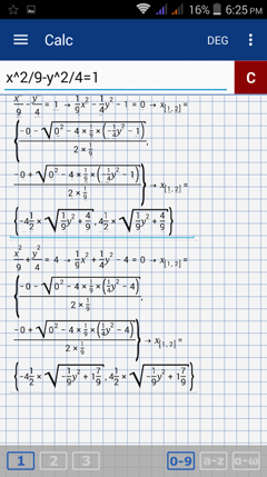
Enter the first equation: x^2/9 - y^2/4 = 1. Type the variable y by tapping the x variable key twice. Hit enter.
Enter the second equation: x^2/9 + y^2/4 = 4.
Note: The calculator displays the values of x in terms of y so it's easier to solve the system by graphing.
Enter the first equation: x^2/9 - y^2/4 = 1. Type the variable y by tapping the x variable key twice. Hit enter.
Enter the second equation: x^2/9 + y^2/4 = 4.
Note: The calculator displays the values of x in terms of y so it's easier to solve the system by graphing.
Solution by Graphing
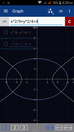
Switch to Graph mode by selecting Graph from the navigation menu.
Enter the first equation: x^2/9 - y^2/4 = 1. Type the variable y by tapping the x variable key twice. Hit enter.
Enter the second equation: x^2/9 + y^2/4 = 4.
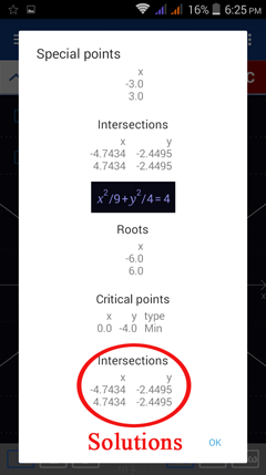
Tap the special points key. Check the "show intersections" option.
Tap "show all."
Note: The points where the graphs intersect represent the solution to the system of equations.
Switch to Graph mode by selecting Graph from the navigation menu.
Enter the first equation: x^2/9 - y^2/4 = 1. Type the variable y by tapping the x variable key twice. Hit enter.
Enter the second equation: x^2/9 + y^2/4 = 4.
Tap the special points key. Check the "show intersections" option.
Tap "show all."
Note: The points where the graphs intersect represent the solution to the system of equations.
Problem 5: Special Case
Algebraic solution
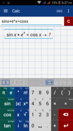
Enter the equation: sinx + e^x = cosx.
Note: The calculator does not display any results but it doesn't mean there is no solution. To solve the system, change the equation into a system of equations: y = sinx + e^x and y = cosx. Find the solution by graphing.
Enter the equation: sinx + e^x = cosx.
Note: The calculator does not display any results but it doesn't mean there is no solution. To solve the system, change the equation into a system of equations: y = sinx + e^x and y = cosx. Find the solution by graphing.
Solution by Graphing
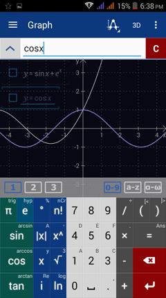
Switch to Graph mode by selecting Graph from the navigation menu.
Enter the right-hand side of the equation: sinx + e^x. Hit enter.
Enter the left-hand side of the equation: cosx.
Tap the special points key. Check the "show intersections" option.
Tap "show all."
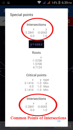
Note: The intersections of each graph are shown. The points of intersection represent the solution set.
Switch to Graph mode by selecting Graph from the navigation menu.
Enter the right-hand side of the equation: sinx + e^x. Hit enter.
Enter the left-hand side of the equation: cosx.
Tap the special points key. Check the "show intersections" option.
Tap "show all."
Note: The intersections of each graph are shown. The points of intersection represent the solution set.