19.6.2. Interquartile Range and Quartile Deviation
Interquartile range (IQR) refers to the range of the middle 50% of a distribution. It can be found by subtracting the third quartile (median of the upper half) and the 1st quartile (median of the lower half), as follows:
|
|
where:
IQR - interquartile range Q3 - third quartile Q1 - 1st quartile |
Finding the IQR requires the following steps:
1) Arrange the data sets from least to highest.
2) Find the values of the 3rd quartile (Q3) and the 1st quartile (Q1) values by using the locator's formula: c = k(n)/4. where k is the quartile and n is the number of values (observations).
Rule of thumb for c
a) If c is a whole number, the quartile value is the average of the values at c and c + 1.
b) If c is not a whole number, the quartile value is the value at the integer when c is rounded off.
3) Subtract Q3 and Q1.
Illustrative Example
Find the IQR of the data set: 12, 4, 5, 6, 9, 10, 8.
Solution
1) Order the data set from lowest to highest.
4, 5, 6, 8, 9, 10, 12
2) Find Q3.
c = 3(7)/4 = 5.25
Round 5.25 off to 5, so Q3 is the 5th value in the set which is 9.
Q3 = 9
3) Find Q1
c = 1(7)/4 = 1.75
Round 1.75 off to 2, so Q1 is the 2nd value in the set which is 5
Q1 = 5
4) IQR = 9 - 5 = 4
Finding the IQR is simple with small data sets, but it is easier to use the app for larger ones.
To find the IQR with the app, use the following steps:
1) Enter the data set as a matrix.
2) Find Q3 by using the syntax: quantile(A, 0.75)
Notes: We use 0.75 for Q3 since it's the value at the 75th percentile of the data.
There is no button for quantiles, so you need to type the command using the a-z keyboard.
3) Find Q1 by using the syntax: quantile (A, 0.25)
Note: We use 0.25 for Q1 since it's the value at the 25th percentile of the data.
4) Find the difference between the results in steps 2 and 3.
Shown below is a demonstration of the calculator syntax:
Examples
Find the IQR for each data set.
1) 12, 4, 5, 6, 7, 9
2) 15, 10, 25, 24, 18, 19
Calculator solutions
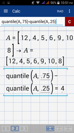
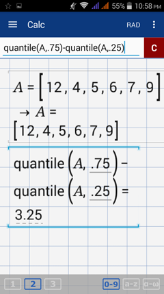
1) Enter the data set as a matrix.
E.g. A = [12, 4, 5, 6, 7, 9]
Find the IQR by using the syntax: quantile(A, 0.75) - quantile(A, 0.25)
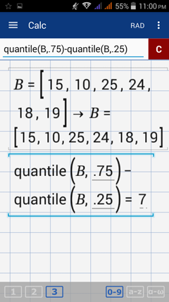
2) Enter the data set as a matrix.
E.g. B = [15, 10, 25, 24, 18, 19]
Find the IQR by using the syntax: quantile(B, 0.75) - quantile(B, 0.25)
Quartile Deviation
The quartile deviation is half of the IQR. It can be found by dividing the IQR by 2.
Use the syntax: (quantile (A, 0.75) - quantile (A, 0.25)) / 2.
Examples
Find the quartile deviation for each data set.
1) 12, 4, 5, 6, 7, 9
2) 15, 10, 25, 24, 18, 19
Calculator solutions
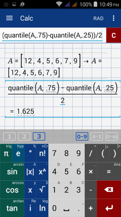
1) Enter the data set as a matrix.
E.g. A = [12, 4, 5, 6, 7, 9]
Find the quartile deviation by using the syntax: (quantile(A, 0.75) - quantile(A, 0.25)) / 2
Use the syntax: (quantile (A, 0.75) - quantile (A, 0.25)) / 2.
Examples
Find the quartile deviation for each data set.
1) 12, 4, 5, 6, 7, 9
2) 15, 10, 25, 24, 18, 19
Calculator solutions
1) Enter the data set as a matrix.
E.g. A = [12, 4, 5, 6, 7, 9]
Find the quartile deviation by using the syntax: (quantile(A, 0.75) - quantile(A, 0.25)) / 2
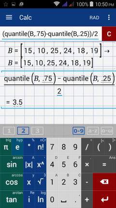
2) Enter the data set as a matrix.
E.g. B = [15, 10, 25, 24, 18, 19]
Find the quartile deviation by using the syntax: (quantile(B, 0.75) - quantile(B, 0.25)) / 2