Get it on Google Play
Graphing Calculator by Mathlab: User Manual
Get it on Google Play
  • Home
    • Introduction
    • PRO Features vs. FREE Version
    • Frequently Asked Questions, FAQs >
      • 1. How to Change the Number Format?
      • 2. How to Set Up the Separators Between Thousands?
      • 3. How to Set Precision?
      • 4. How to Send Feedback with Comments?
      • 5. How to import/export the library?
      • 6. How to Print Results?
      • 7. How to Make the Calculator Show the Results?
      • 8. How to Transport Calculation Results to other Programs?
      • 9. How to Transport Table to Other Platforms?
      • 10. How to Turn Off (or on) Vibration?
      • 11. How to Change the Language?
  • 1. Basics
    • 1.1. Navigation
    • 1.2. UI Elements
    • 1.3. Keyboard
    • 1.4. Input, Enter, Delete, Clear and UNDO Buttons
    • 1.5. Workspace Area
    • 1.6. Editing the Expression/Equation
    • 1.7. Using the Last Answer
    • 1.8. Writing Comments
    • 1.9. Clear, Copy & Paste Commands
    • 1.10. Rearranging Rows
  • 2. Settings
    • 2.1. General
    • 2.2. Calculator
    • 2.3. Graph
  • 3. Library
    • 3.1. Constants
    • 3.2. Functions
    • 3.3. How to Save Calculation Result/Graph to Library?
  • 4. Graph Mode
    • 4.1. 2D Graphing
    • 4.2. 3D Graphing
    • 4.3. Enlarging the Graph Area
    • 4.4. Changing to White Background
    • 4.5. Hide Keyboard
    • 4.6. Degree and Radian Scales
    • 4.7. Fixed Scale
    • 4.8. R-axis Scale
    • 4.9. Logarithmic Scale
    • 4.10. Tracing Values and Slopes
    • 4.11. Special Points: Roots and Criticals
    • 4.12. Intersections of Graphs
    • 4.13. Set Domain
    • 4.14. Show All - Roots, Critical Points and Intersections
    • 4.15. Fullscreen
  • 5. Table Mode
    • 5.1. Sharing of Functions
    • 5.2. 2D Table
    • 5.3. 3D Table
    • 5.4. Edit Functions
    • 5.5. Scroll Results
    • 5.6. Results Precision
    • 5.7. Zoom Controls
    • 5.8. Save and Load Table
    • 5.9. Table of Trigonometric Functions
  • 6. Numbers and Number Sense
    • 6.1. Decimals
    • 6.2. Fractions >
      • 6.2.1. Mixed Fractions
      • 6.2.2. Complex Fractions
      • 6.2.3. Converting Decimals to Fractions
      • 6.2.4. Converting Fractions to Decimals
    • 6.3. Percents
    • 6.4. Scientific Notation
    • 6.5. Engineering Notation
    • 6.6. Rounding Numbers
    • 6.7. Integer and Fractional Parts >
      • 6.7.1. Integer Part of a Number >
        • 6.7.1.1. Ceiling
        • 6.7.1.2. Floor
        • 6.7.1.3. Half Down
        • 6.7.1.4. Half to Even
        • 6.7.1.5. Half to Infinity
        • 6.7.1.6. Half to Odd
        • 6.7.1.7. Half to Zero
        • 6.7.1.8. Half Up
        • 6.7.1.9. Truncate
      • 6.7.2. Greatest Integer is the Floor Function
      • 6.7.3. Least Integer is the Ceiling Function
      • 6.7.4. Fractional Part of a Number
    • 6.8. Order of Operations
    • 6.9. Least Common Multiple
    • 6.10. Greatest Common Divisor
    • 6.11. Modulo
    • 6.12. Binary, Octal, Decimal, Hexadecimal Numbers
    • 6.13. Complex Numbers
    • 6.14. The Polar Form of Complex Numbers
    • 6.15. Polar to Rectangular Coordinates
  • 7. Introductory Algebra
    • 7.1. Arithmetic Operations
    • 7.2. Exponents
    • 7.3. Absolute Values
    • 7.4. Variables
    • 7.5. Evaluating Expressions
    • 7.6. Polynomials
    • 7.7. Roots
    • 7.8. Logarithms
  • 8. Equations in One Variable
    • 8.1. Linear Equation
    • 8.2. Absolute Value Equation
    • 8.3. Quadratic Equation
    • 8.4. Cubic Equation
    • 8.5. Polynomial Equation
    • 8.6. Rational Equation
    • 8.7. Radical Equation
    • 8.8. Exponential Equation
    • 8.9. Logarithmic Equation
  • 9. Inequalities in One Variable
    • 9.1. Inequality Symbols
    • 9.2. Linear Inequalities
    • 9.3. Absolute Value Inequalities
    • 9.4. Quadratic Inequality
    • 9.5. Polynomial Inequalities
    • 9.6. Rational Inequalities
    • 9.7. Compound Inequalities
    • 9.8. Inequalities with Constants
  • 10. Equations and Inequalities in Two Variables
    • 10.1. Linear Equations
    • 10.2. Systems of Linear Equations
    • 10.3. Graphing Inequalities
    • 10.4. Multiple Graphing of Inequalities
    • 10.5. Graphing Systems of Inequalities
    • 10.6. Solving Implicit Equations
  • 11. Algebraic Functions and Graphs
    • 11.1. Plotting Points
    • 11.2. How to Graph Functions?
    • 11.3. Setting the Applied Domain
    • 11.4. Linear Function
    • 11.5. Absolute Value Function
    • 11.6. Quadratic Function
    • 11.7. Polynomial Functions
    • 11.8. Rational Functions
    • 11.9. Radical Functions
    • 11.10. Logarithmic Functions
    • 11.11. Exponential Functions
    • 11.12. Sign Function
    • 11.13. Multiple Graphing
    • 11.14. Piecewise Functions
  • 12. Matrices and Vectors
    • 12.1. Matrix Operations
    • 12.2. Editing Matrix Entries
    • 12.3. Matrix Variables
    • 12.4. Matrix and Vector Forms
    • 12.5. Variable Matrix to System of Linear Equations
    • 12.6. Solving Systems of Linear Equations Using Matrix Equations
  • 13. Trigonometric Functions and Their Inverses
    • 13.1. Degrees and Radians >
      • 13.1.1. Degrees, Minutes and Seconds
      • 13.1.2. Bradis Table
    • 13.2. Trigonometric Function Keys
    • 13.3. Trigonometric Values of Special Angles >
      • 13.3.1. The 45- 45 - 90 Triangle
      • 13.3.2. The 30-60-90 Triangle
      • 13.3.3. Quadrantal Angles
      • 13.3.4. Coterminal Angles
    • 13.4. Trigonometric Values of 15 Degrees and Its Multiples
    • 13.5. Hyperbolic Function Keys
    • 13.6. Graphing Trigonometric Functions
    • 13.7. Graphing Hyperbolic Functions
    • 13.8. Graphing Inverse Functions
  • 14. Analytic Geometry
    • 14.1. Conic Sections
    • 14.2. Parametric Equations
    • 14.3. Polar Graphs >
      • 14.3.1. Limacon
      • 14.3.2. Cardioid
      • 14.3.3. Lemniscate
      • 14.3.4. Rose
      • 14.3.5. Other Polar Graphs
    • 14.4. 3D Graphing
  • 15. Limits
    • 15.1. Right - hand Limit
    • 15.2. Left - hand Limit
    • 15.3. Limit of a Function
    • 15.4. Limit of a Polynomial Function
    • 15.5. Limit of a Rational Function
    • 15.6. Limit of a Radical Function
    • 15.7. Limit of an Absolute Value Function
    • 15.8. Limit of a Trigonometric Function
    • 15.9. Limit of an Exponential and Logarithmic Function
    • 15.10. Limit of a Piece-wise Function
    • 15.11. Limits at Infinity
    • 15.12. Indeterminate Forms
    • 15.13. Limit of a Hyperbolic Function
  • 16. Derivatives
    • 16.1. First Derivative Key
    • 16.2. Second Derivative Key
    • 16.3. Third and Higher Derivative Keys
    • 16.4. Rules of Differentiation
    • 16.5. Derivatives of Polynomial Functions
    • 16.6. Derivatives of Rational Functions
    • 16.7. Dervatives of Trigonometric, Logarithmic and and Exponential Functions
    • 16.8. More on Derivatives
  • 17. Partial Derivatives
    • 17.1. Increments
    • 17.2. Dervative of a Function df (or dy))
    • 17.3. Derivative of a Function df (f not in terms of x)
    • 17.4. Other Partial Derivatives
    • 17.5. Higher Order Partial Derivatives
    • 17.6. Total Derivates
  • 18. Definite Integral
    • 18.1. Definite Integral of Algebraic Functions
    • 18.2. Definite Integral of Trigonometric Functions
  • 19. Basic Statistics
    • 19.1. Summation Notation
    • 19.2. Product Notation
    • 19.3. Minimum and Maximum
    • 19.4. Factorial, nCr and nPr
    • 19.5. Measures of Central Tendency >
      • 19.5.1. Mean from Ungrouped Data Set
      • 19.5.2. Mean from Frequency Distribution Table
      • 19.5.3. Median from Ungrouped Data Set
      • 19.5.4. Mode
    • 19.6. Measures of Variability >
      • 19.6.1. Range
      • 19.6.2. Interquartile Range and Quartile Deviation
      • 19.6.3. Mean Absolute Deviation
      • 19.6.4. Variance and Standard Deviation
      • 19.6.5. Coefficient of Variation
    • 19.7. Measures of Position
    • 19.8. Bivariate Data Analysis >
      • 19.8.1 Covariance
      • 19.8.2. Correlation Coefficient
      • 19.8.3. Scatter Plot and Regression Line
  • 20. Special Functions
    • 20.1. Gamma Function
    • 20.2. Logarithmic Gamma Function
    • 20.3. Digamma Function
  • 21. List of ALL Functions
    • 21.1. Arithmetics
    • 21.2. Algebra
    • 21.3. Trigonometry
    • 21.4. Statistics
    • 21.5. Calculus

19.6.5. Coefficient of Variation

The coefficient of variation (CV) is used to compare the variability of two data sets with either the same or different units such as ticket sales to the number of tickets sold or the prices of a commodity to the quantity sold. CV is the percentage equivalent of the standard deviation relative to the mean of the distribution.

To calculate the CV, divide the standard deviation by the mean and multiply the result by 100%. When comparing data sets, a larger CV implies higher variability.

Illustrative Example
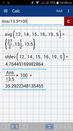
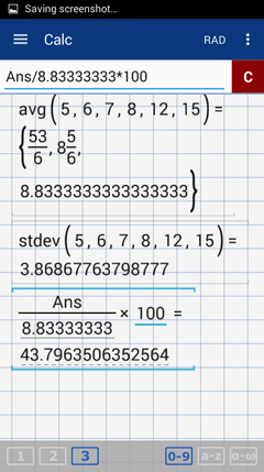
Which data set has more variability?
Data set A:  12, 14, 15, 16, 19, 5
Data set B: 5, 6, 7, 8, 12, 15

Solution
Find the mean and standard deviation of each data set. 

Data set A                                                       Data Set B
Mean =  13.5                                                    Mean = 8.83333333
Standard deviation = 4.76445169               Standard deviation = 3.868677638

Calculate the CV
Data set A: CV = s.d. / mean = 35.2922348%
Data set B: CV = s.d. / mean = 43.7963506%

Because set B has a higher CV, its values have a higher variability than the values in set A.
Picture
Picture

Calculator solution
Enter each data set as matrix.
    E.g.  A = [12, 14, 15, 16, 19, 5] ;  B = [5, 6, 7, 8, 12, 15]
Use the syntax: stdev(A)/avg(A) × 100 to find the CV of data set A and stdev(B)/avg(B) × 100 to find the CV of data set B.

Note: If the data set represents a population of values, use stdevp for the standard deviation.
Picture

Examples

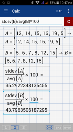
1) Samples of 10 math scores were taken from classes A and B respectively. Determine which class's math scores have less variability.
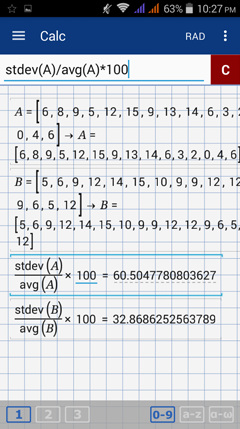
    Class A: 6, 8, 9, 5, 12, 15, 9, 13, 14, 6, 3, 2, 0, 4, 6
    Class B: 5, 6, 9, 12, 14, 15, 10, 9, 9, 12, 12, 9, 6, 5, 12

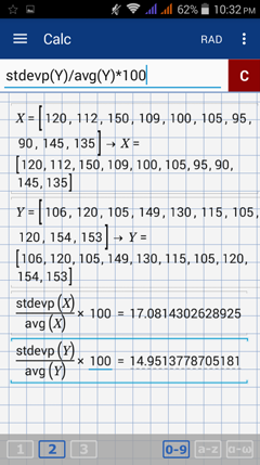
2) The weights (in pounds) of all 10 supervisors and managers at two companies are listed below. Which weights have more                        variability?
     Company X:  120, 112, 150, 109, 100, 105, 95, 90, 145, 135
     Company Y:  106, 120, 105, 149, 130, 115, 105, 120, 154, 153

Calculator solutions
1) Enter the data sets in matrix form.
    E.g.  A = [6, 8, 9, 5, 12, 15, 9, 13, 14, 6, 3, 2, 0, 4, 6] , B = [5, 6, 9, 12, 14, 15, 10, 9, 9, 12, 12, 9, 6, 5, 12]
    Find the CV for data set A using the syntax: stdev(A)/avg(A) × 100 
    Compute the CV for data set B using the syntax: stdev(B)/avg(B) × 100 

Since the CV for the math scores in class B (32.87%) is less than the CV in class A (60.50%), data set B has less variability.
Picture

2) Enter the data sets in matrix form.
    E.g.  X = [120, 112, 150, 109, 100, 105, 95, 90, 145, 135] , Y = [106, 120, 105, 149, 130, 115, 105, 120, 154, 153]
    Find the CV for data set A using the syntax: stdevp(X)/avg(X) × 100 
    Find the CV for data set B using the syntax: stdevp(Y)/avg(Y) × 100 

Since the CV for company X (17.08%) is higher than the CV for company Y (14.95%), company X has more variability in the weights of its supervisors and managers.
Picture
NEXT: 19.7. measures of position >
list of contents
Powered by Create your own unique website with customizable templates.