Get it on Google Play
Graphing Calculator by Mathlab: User Manual
Get it on Google Play
  • Home
    • Introduction
    • PRO Features vs. FREE Version
    • Frequently Asked Questions, FAQs >
      • 1. How to Change the Number Format?
      • 2. How to Set Up the Separators Between Thousands?
      • 3. How to Set Precision?
      • 4. How to Send Feedback with Comments?
      • 5. How to import/export the library?
      • 6. How to Print Results?
      • 7. How to Make the Calculator Show the Results?
      • 8. How to Transport Calculation Results to other Programs?
      • 9. How to Transport Table to Other Platforms?
      • 10. How to Turn Off (or on) Vibration?
      • 11. How to Change the Language?
  • 1. Basics
    • 1.1. Navigation
    • 1.2. UI Elements
    • 1.3. Keyboard
    • 1.4. Input, Enter, Delete, Clear and UNDO Buttons
    • 1.5. Workspace Area
    • 1.6. Editing the Expression/Equation
    • 1.7. Using the Last Answer
    • 1.8. Writing Comments
    • 1.9. Clear, Copy & Paste Commands
    • 1.10. Rearranging Rows
  • 2. Settings
    • 2.1. General
    • 2.2. Calculator
    • 2.3. Graph
  • 3. Library
    • 3.1. Constants
    • 3.2. Functions
    • 3.3. How to Save Calculation Result/Graph to Library?
  • 4. Graph Mode
    • 4.1. 2D Graphing
    • 4.2. 3D Graphing
    • 4.3. Enlarging the Graph Area
    • 4.4. Changing to White Background
    • 4.5. Hide Keyboard
    • 4.6. Degree and Radian Scales
    • 4.7. Fixed Scale
    • 4.8. R-axis Scale
    • 4.9. Logarithmic Scale
    • 4.10. Tracing Values and Slopes
    • 4.11. Special Points: Roots and Criticals
    • 4.12. Intersections of Graphs
    • 4.13. Set Domain
    • 4.14. Show All - Roots, Critical Points and Intersections
    • 4.15. Fullscreen
  • 5. Table Mode
    • 5.1. Sharing of Functions
    • 5.2. 2D Table
    • 5.3. 3D Table
    • 5.4. Edit Functions
    • 5.5. Scroll Results
    • 5.6. Results Precision
    • 5.7. Zoom Controls
    • 5.8. Save and Load Table
    • 5.9. Table of Trigonometric Functions
  • 6. Numbers and Number Sense
    • 6.1. Decimals
    • 6.2. Fractions >
      • 6.2.1. Mixed Fractions
      • 6.2.2. Complex Fractions
      • 6.2.3. Converting Decimals to Fractions
      • 6.2.4. Converting Fractions to Decimals
    • 6.3. Percents
    • 6.4. Scientific Notation
    • 6.5. Engineering Notation
    • 6.6. Rounding Numbers
    • 6.7. Integer and Fractional Parts >
      • 6.7.1. Integer Part of a Number >
        • 6.7.1.1. Ceiling
        • 6.7.1.2. Floor
        • 6.7.1.3. Half Down
        • 6.7.1.4. Half to Even
        • 6.7.1.5. Half to Infinity
        • 6.7.1.6. Half to Odd
        • 6.7.1.7. Half to Zero
        • 6.7.1.8. Half Up
        • 6.7.1.9. Truncate
      • 6.7.2. Greatest Integer is the Floor Function
      • 6.7.3. Least Integer is the Ceiling Function
      • 6.7.4. Fractional Part of a Number
    • 6.8. Order of Operations
    • 6.9. Least Common Multiple
    • 6.10. Greatest Common Divisor
    • 6.11. Modulo
    • 6.12. Binary, Octal, Decimal, Hexadecimal Numbers
    • 6.13. Complex Numbers
    • 6.14. The Polar Form of Complex Numbers
    • 6.15. Polar to Rectangular Coordinates
  • 7. Introductory Algebra
    • 7.1. Arithmetic Operations
    • 7.2. Exponents
    • 7.3. Absolute Values
    • 7.4. Variables
    • 7.5. Evaluating Expressions
    • 7.6. Polynomials
    • 7.7. Roots
    • 7.8. Logarithms
  • 8. Equations in One Variable
    • 8.1. Linear Equation
    • 8.2. Absolute Value Equation
    • 8.3. Quadratic Equation
    • 8.4. Cubic Equation
    • 8.5. Polynomial Equation
    • 8.6. Rational Equation
    • 8.7. Radical Equation
    • 8.8. Exponential Equation
    • 8.9. Logarithmic Equation
  • 9. Inequalities in One Variable
    • 9.1. Inequality Symbols
    • 9.2. Linear Inequalities
    • 9.3. Absolute Value Inequalities
    • 9.4. Quadratic Inequality
    • 9.5. Polynomial Inequalities
    • 9.6. Rational Inequalities
    • 9.7. Compound Inequalities
    • 9.8. Inequalities with Constants
  • 10. Equations and Inequalities in Two Variables
    • 10.1. Linear Equations
    • 10.2. Systems of Linear Equations
    • 10.3. Graphing Inequalities
    • 10.4. Multiple Graphing of Inequalities
    • 10.5. Graphing Systems of Inequalities
    • 10.6. Solving Implicit Equations
  • 11. Algebraic Functions and Graphs
    • 11.1. Plotting Points
    • 11.2. How to Graph Functions?
    • 11.3. Setting the Applied Domain
    • 11.4. Linear Function
    • 11.5. Absolute Value Function
    • 11.6. Quadratic Function
    • 11.7. Polynomial Functions
    • 11.8. Rational Functions
    • 11.9. Radical Functions
    • 11.10. Logarithmic Functions
    • 11.11. Exponential Functions
    • 11.12. Sign Function
    • 11.13. Multiple Graphing
    • 11.14. Piecewise Functions
  • 12. Matrices and Vectors
    • 12.1. Matrix Operations
    • 12.2. Editing Matrix Entries
    • 12.3. Matrix Variables
    • 12.4. Matrix and Vector Forms
    • 12.5. Variable Matrix to System of Linear Equations
    • 12.6. Solving Systems of Linear Equations Using Matrix Equations
  • 13. Trigonometric Functions and Their Inverses
    • 13.1. Degrees and Radians >
      • 13.1.1. Degrees, Minutes and Seconds
      • 13.1.2. Bradis Table
    • 13.2. Trigonometric Function Keys
    • 13.3. Trigonometric Values of Special Angles >
      • 13.3.1. The 45- 45 - 90 Triangle
      • 13.3.2. The 30-60-90 Triangle
      • 13.3.3. Quadrantal Angles
      • 13.3.4. Coterminal Angles
    • 13.4. Trigonometric Values of 15 Degrees and Its Multiples
    • 13.5. Hyperbolic Function Keys
    • 13.6. Graphing Trigonometric Functions
    • 13.7. Graphing Hyperbolic Functions
    • 13.8. Graphing Inverse Functions
  • 14. Analytic Geometry
    • 14.1. Conic Sections
    • 14.2. Parametric Equations
    • 14.3. Polar Graphs >
      • 14.3.1. Limacon
      • 14.3.2. Cardioid
      • 14.3.3. Lemniscate
      • 14.3.4. Rose
      • 14.3.5. Other Polar Graphs
    • 14.4. 3D Graphing
  • 15. Limits
    • 15.1. Right - hand Limit
    • 15.2. Left - hand Limit
    • 15.3. Limit of a Function
    • 15.4. Limit of a Polynomial Function
    • 15.5. Limit of a Rational Function
    • 15.6. Limit of a Radical Function
    • 15.7. Limit of an Absolute Value Function
    • 15.8. Limit of a Trigonometric Function
    • 15.9. Limit of an Exponential and Logarithmic Function
    • 15.10. Limit of a Piece-wise Function
    • 15.11. Limits at Infinity
    • 15.12. Indeterminate Forms
    • 15.13. Limit of a Hyperbolic Function
  • 16. Derivatives
    • 16.1. First Derivative Key
    • 16.2. Second Derivative Key
    • 16.3. Third and Higher Derivative Keys
    • 16.4. Rules of Differentiation
    • 16.5. Derivatives of Polynomial Functions
    • 16.6. Derivatives of Rational Functions
    • 16.7. Dervatives of Trigonometric, Logarithmic and and Exponential Functions
    • 16.8. More on Derivatives
  • 17. Partial Derivatives
    • 17.1. Increments
    • 17.2. Dervative of a Function df (or dy))
    • 17.3. Derivative of a Function df (f not in terms of x)
    • 17.4. Partial Derivatives
    • 17.5. Higher Order Partial Derivatives
    • 17.6. Total Derivates
  • 18. Definite Integral
    • 18.1. Definite Integral of Algebraic Functions
    • 18.2. Definite Integral of Trigonometric Functions
  • 19. Basic Statistics
    • 19.1. Summation Notation
    • 19.2. Product Notation
    • 19.3. Minimum and Maximum
    • 19.4. Factorial, nCr and nPr
    • 19.5. Measures of Central Tendency >
      • 19.5.1. Mean from Ungrouped Data Set
      • 19.5.2. Mean from Frequency Distribution Table
      • 19.5.3. Median from Ungrouped Data Set
      • 19.5.4. Mode
    • 19.6. Measures of Variability >
      • 19.6.1. Range
      • 19.6.2. Interquartile Range and Quartile Deviation
      • 19.6.3. Mean Absolute Deviation
      • 19.6.4. Variance and Standard Deviation
      • 19.6.5. Coefficient of Variation
    • 19.7. Measures of Position
    • 19.8. Bivariate Data Analysis >
      • 19.8.1 Covariance
      • 19.8.2. Correlation Coefficient
      • 19.8.3. Scatterplot and Regression Line
  • 20. Special Functions
    • 20.1. Gamma Function
    • 20.2. Logarithmic Gamma Function
    • 20.3. Digamma Function
  • 21. List of ALL Functions
    • 21.1. Arithmetics
    • 21.2. Algebra
    • 21.3. Trigonometry
    • 21.4. Statistics
    • 21.5. Calculus

19.6.4. Variance and Standard Deviation

Variance and standard deviation are the most common measures of spread in statistical hypothesis tests. Variance refers to the average of the squared differences between each data value and the mean, and standard deviation is the square root of the variance. Variance is expressed in squared units while standard deviation is expressed in the same units as the data values.

Calculating the Variance and Standard Deviation of Ungrouped Data Sets

To find the variance and standard deviation:
1) Find the mean of the data set.
2) Subtract the mean from each data value.
3) Take the square of each difference.
4) Find the average of the squared differences, but divide by (n - 1) if the data came from a sample. Divide by n if the data set is the population. The average is the value of the variance.
5) Take the square root of the variance to get the standard deviation.

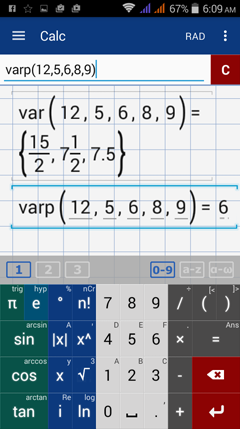
Illustrative Example
Find the variance and standard deviation of the data set.
12, 5, 6, 8, 9

Solution
1) Find the average of the data values.
    average = (12 + 5 + 6 + 8 + 9)/5 = 8

2) Subtract the mean from each data value.
     X                  X - Mean
    12                       4
     5                      -3
     6                      -2
     8                       0
     9                        1

3) Square each difference.
     X                  X - Mean               (X - Mean)^2
    12                       4                                     16
     5                      -3                                     9
     6                      -2                                     4
     8                       0                                     0
     9                        1                                       1

4)  Find the average of the squared differences.
     Population variance = (16 + 9 + 4 + 0 + 1)/5 = 6  
     Sample variance = (16 + 9 + 4 + 0 + 1)/ (5 - 1) = 7.5

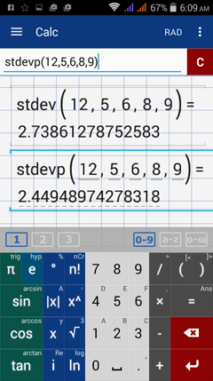
5) Take the square root of the variance to find the standard deviation.
     Population standard deviation = square root (6) = 2.4494897
     Sample standard deviation = square root (7.5) = 2.738612787

The manual calculations of the variance and standard deviation are simple for small data sets, but it is easier to use the app for data sets that are large. The values for the variance and standard deviation can be found by using var and stdev for sample data or varp and setdevp for population data respectively.
Picture
Picture

Examples

Calculate the variance and standard deviation of each data set below.

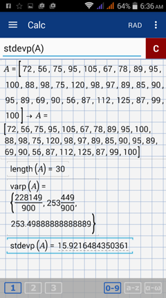
1) The heights (in inches) of all 30 employees at a manufacturing company are listed below.
    72, 56, 75, 95, 105, 67, 78, 89, 95, 100, 88, 98, 75, 120, 98, 97, 89, 85, 90, 95, 89, 69, 90, 56, 87, 112, 125, 87, 99, 100

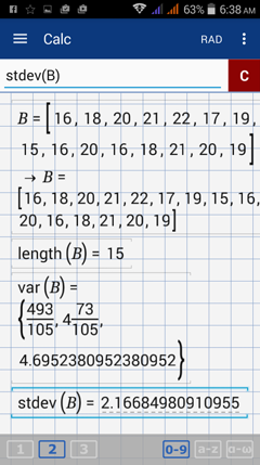
2) The ages in years of 15 randomly selected students at a college are as follows:
    16, 18, 20, 21, 22, 17, 19, 15, 16, 20, 16, 18, 21, 20, 19

Calculator solutions
1) Since the data set contains the heights for all 30 employees, the data set represents a population so we use varp for variance and stdevp for standard deviation.
   a) Calculating the population variance
       Enter the data set as a matrix. Use brackets and separate data values with a comma.
       E.g. A = [72, 56, 75, 95, 105, 67, 78, 89, 95, 100, 88, 98, 75, 120, 98, 97, 89, 85, 90, 95, 89, 69, 90, 56, 87, 112, 125, 87, 99, 100]

Note: To check if you entered all of the data values, you can find the length of the data set by entering length(A). Select "length" by holding the factorial (n!) key. 

       Hold the factorial (n!) key and select varp. Type the name of the matrix, A.
       E.g. varp(A)
      
   b) Calculating the population standard deviation.
        Since the data set has already been entered as a matrix, you can refer to it by its matrix name, A in this case.
        To calculate the standard deviation, hold the factorial (n!) key and select stdevp. Enter the matrix in parentheses.
        E.g. stdevp(A)
Picture

2) Since the data set is composed of the ages of a select number of students at the college, it represents a sample of values. In this case, we use the commands var for variance and stdev for standard deviation.
   a) Calculating the sample variance
       Enter the data set as a matrix. Use brackets and separate data values with a comma.
       E.g. B = [16, 18, 20, 21, 22, 17, 19, 15, 16, 20, 16, 18, 21, 20, 19]

Note: To check if you entered all of the data values, you can find the length of the data set by entering length(A). Select "length" by holding the factorial (n!) key.​

       Hold the factorial (n!) key and select var. Type the name of the matrix, B.
       E.g. var(B)       

   b) Calculating the sample standard deviation.
        Since the data set has already been entered as a matrix, you can refer to it by its matrix name, B in this case.
        To calculate the standard deviation, hold the factorial (n!) key and select stdev. Enter the matrix in parentheses.
        E.g. stdev(B)
Picture
NEXT: 19.6.5. COEFFICIENT OF VARIATION >
list of contents
Powered by Create your own unique website with customizable templates.